HUBS Galactic Ecosystems SWG · Science China paper · Fig. 3

Updated figure of merit comparison

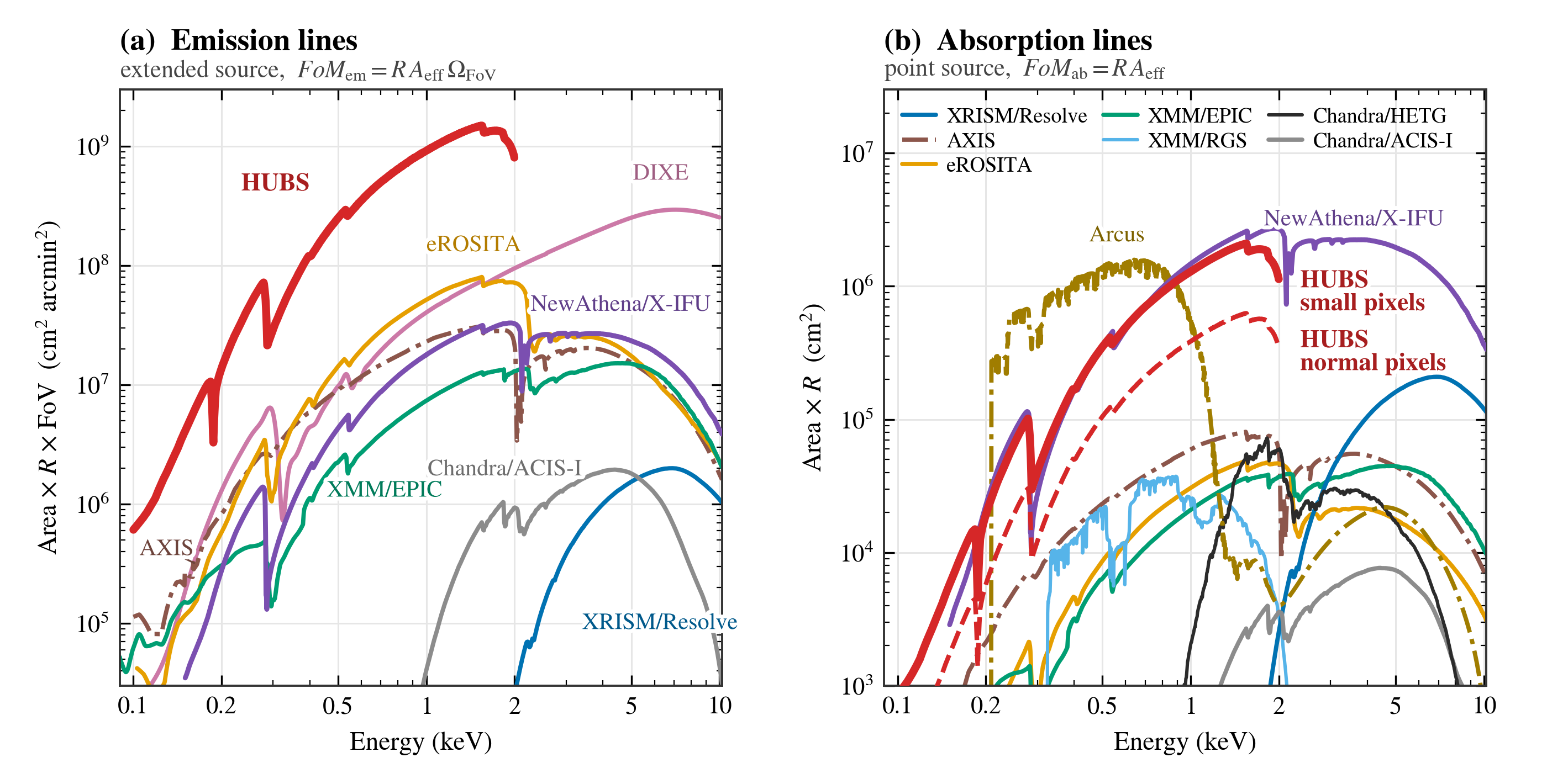
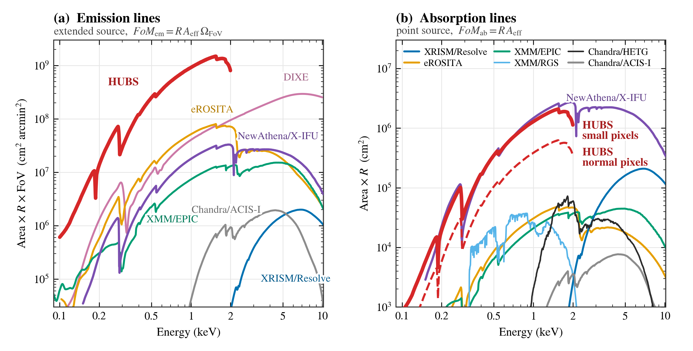
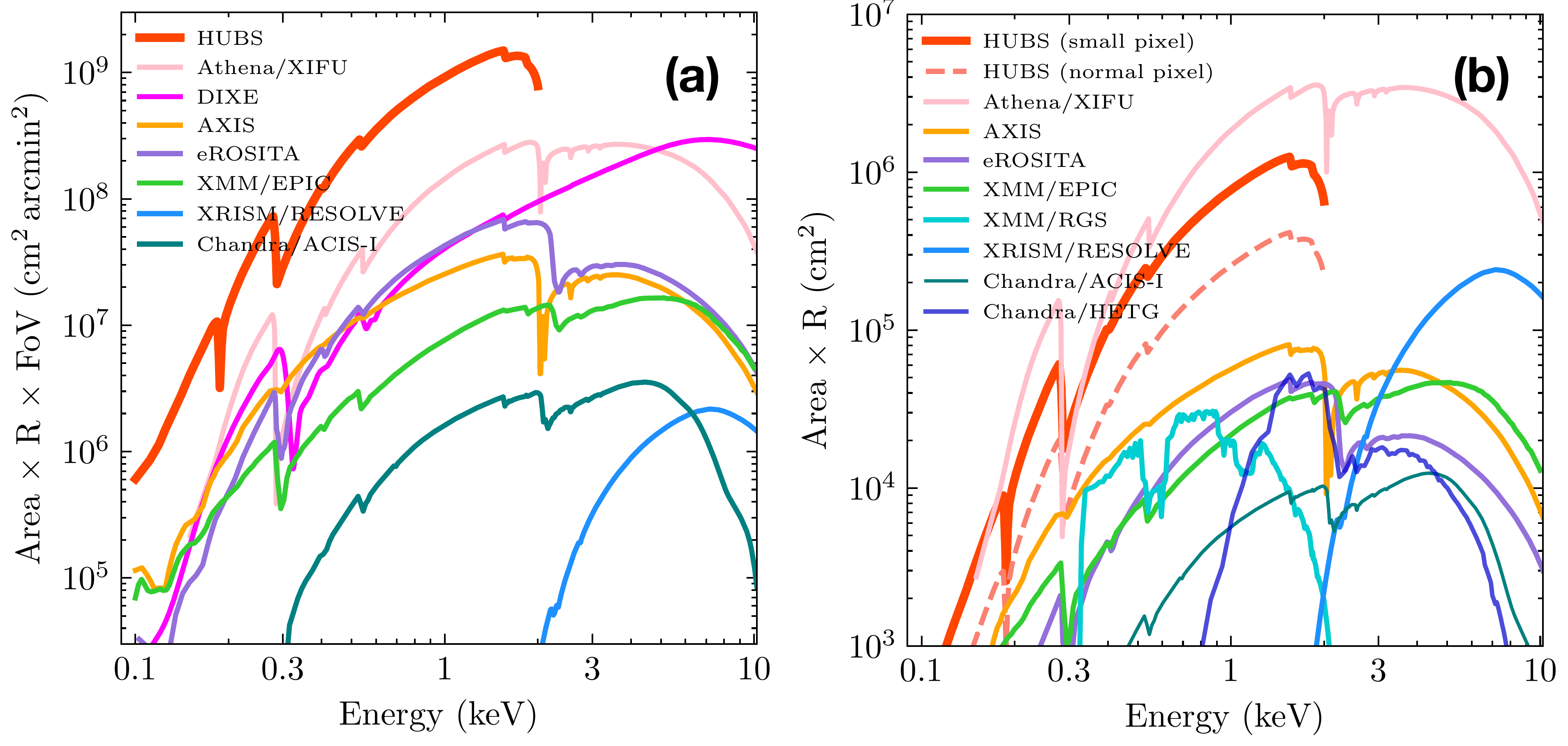
Fig. 3 compares how well X-ray missions detect weak emission lines from extended hot gas, panel (a), and absorption lines against point sources, panel (b). We rebuilt it from the current public responses of every instrument. Two versions are offered for the paper: one with all missions, and one without the NASA Probe concepts AXIS and Arcus, which were not selected for flight.

≈50×(a) At 1 keV, HUBS exceeds NewAthena/X-IFU by about 50× (previous figure: about 6×). X-IFU now uses its real 12.3 arcmin² field of view and the 4 eV baseline resolution.

≈18×(a) At 1 keV, HUBS exceeds the next-best instrument, eROSITA, by about 18×. Removing AXIS does not change any ranking in (a).

0.2–0.9 keV(b) The Arcus 2021 design is the highest curve in this range. Without Arcus, HUBS small pixels and X-IFU lead together, within ±15% of each other between 0.35 and 1 keV.

×0.03Chandra/ACIS-I at 1 keV, new/previous. The previous curve used an ACIS-S3 response without the contamination layer; the new one uses ACIS-I Cycle 28.

Two versions for the paper

The two versions differ in only one way: the AXIS and Arcus curves are removed, together with their entries in the (b) legend and the caption. All other curves are identical. Switch between them to see what drops out.

(a) Emission lines

Only AXIS disappears. It sat below eROSITA and DIXE at all energies, so the order of the remaining curves is unchanged: HUBS leads the next instrument by about 18× over 0.5–1.5 keV.

(b) Absorption lines

Arcus was the top curve from 0.21 to 0.88 keV, up to 11× above HUBS small pixels. Without it, HUBS small pixels and X-IFU are the top two below 2 keV and trade places within ±15% between 0.35 and 1 keV.

Caption

The full version adds “Dash-dotted curves mark the concept missions not selected for flight (AXIS and Arcus)” and lists their responses. The other version drops Arcus from the list of summed orders and AXIS from the list of responses.

Previous figure vs new figure

Left: the figure currently in the manuscript (FoM_merge_v5.pdf). Right: the new figure, with all missions. The new figure is also redrawn: each curve is labelled directly, each instrument keeps one colour, and the panels are titled by line type.

Previous Fig. 3: (a) Area×R×FoV, (b) Area×R — Previous (2025-02, in the manuscript)

New Fig. 3 with all missions — New (2026-10), all missions

Instrument by instrument

Each small chart shows one instrument, on the same y-range as the paper figure. Hover or tap to read both versions and their ratio at any energy. The chips give new/previous at 0.5, 1 and 6 keV.

newprevious

What changed, per instrument

Instrument	Previous figure	New figure	Effect
HUBS	Normal pixels 2 eV, small pixels 1 eV; (b) normal pixels used the vignetted (FoV-averaged) ARF	Small pixels 0.6 eV (Cui et al. 2020); in (b) both pixel types use the on-axis ARF, in (a) the vignetted ARF	(a) unchanged; (b) small ×1.67, normal ×1.51
NewAthena/X-IFU	2024-04 responses, 3 eV (design goal), optical filter; FoV π·5′² = 78.5 arcmin²	2026-05 Mission Adoption Review release, 4 eV baseline, filter wheel open; 1504-pixel hexagon (12.3 arcmin²) with ESA vignetting	(a) ×0.12 at 1 keV; (b) ×0.80
XMM/EPIC	Older RMFs and on-axis ARFs; FoV π·15′² × 0.5; combined as (ΣA)²/Σ(A/R)	Canned RMFs (MOS e19, pn e4 v22); on-axis Thin ARFs from `arfgen` for 2026-10-01; FoV integral of the CCF vignetting (MOS1 without CCD3/6); Σ R·A	≈ unchanged at 1 keV; ×0.38 at 0.3 keV (MOS contamination, pn redistribution)
XMM/RGS	SAS v18 matrices; earlier R method	SAS v21 matrices; R from the measured FWHM, dead-CCD rows skipped; Σ R·A over RGS1/2, orders 1/2	×1.27 at 1 keV, ×1.6 at 1.5 keV
XRISM/Resolve	2019 RMF with the gate-valve-closed ARF; FoV 3′×3′	Cycle 3 responses (gate valve closed, 4.5 eV); (a) uses the 5′-radius flat-source ARF × π·5′²	≈ unchanged at 6 keV
Chandra/ACIS-I	Labelled ACIS-I, but actually an ACIS-S3 response without contamination	Cycle 28 ACIS-I aimpoint (contamination to 2027-05); HRMA vignetting over the 16.9′ field	×0.03 at 1 keV, ×0.54 at 6 keV
Chandra/HETG	Cycle 23, HEG/MEG ±1 only, FWHM rounded to whole channels	Cycle 28, HEG/MEG ±1, ±2, ±3, measured FWHM, Σ R·A	×0.33 at 1 keV (contamination), ×1.68 at 6 keV
eROSITA	π·30′² × 0.5	SIXTE vignetting of all 7 telescope modules with the CALDB field maps	(a) ×1.2
AXIS	On-axis ARF × 450 arcmin²	FoV-averaged ARF × π·12′²	(a) ×0.86–0.91
DIXE	Unchanged: 6 eV, collimator effective FoV 87.5 deg²		—
Arcus	Not plotted, although the caption mentioned it	2021 design: far-camera orders −2 to −11 (order-sorted ARFs) plus zeroth order; near-camera orders have no ARFs in that release	new

Three method changes

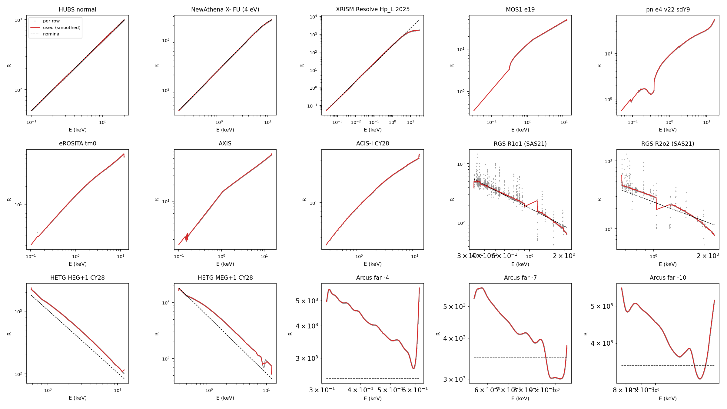
R is measured from each response matrix

The previous figure fitted a Gaussian in channel space, then converted channels to energy with a polynomial and smoothed ΔE with another polynomial. That is good to a few per cent for CCDs and calorimeters, but it gave R too low by about 1.5× for RGS at 1.5 keV and rounded the HETG width to whole channels. Now each matrix row is placed on its true EBOUNDS energies, and the FWHM is read from the half-maximum crossings. If a CCD gap cuts one wing of the line, twice the other half-width is used. The chart below compares the result with published nominal values. HUBS, X-IFU and XRISM match exactly and RGS agrees to 10–20%. HETG comes out about 25% higher than the POG nominal value, which is a property of the CXC grating matrices themselves.

R(E) per instrument: row-by-row measurement, adopted curve, published nominal value — Grey points: row-by-row FWHM measurement; red: adopted R; black dashed: published nominal value.

Several detectors or orders: Σ R·A

For a weak unresolved line, the S/N² of one spectrum is proportional to R·A·t, and the S/N² of independent spectra adds. So the combined FoM is Σ R_iA_i. The previous formula, (ΣA)²/Σ(A/R), is equivalent to merging the spectra into one with an area-weighted ΔE. It is never larger than the sum (Cauchy–Schwarz), and for HETG it was about 9% lower at 1 keV.

(a) Uses the FoV-integrated area for every telescope

A·Ω in FoM_em becomes ∫A(E,θ)dΩ, the grasp. The vignetted solid angle ∫V dΩ at 1 keV is 290 (MOS1), 385 (MOS2), 363 (pn), 1692 (eROSITA), 262 (ACIS-I) and 12.1 (X-IFU) arcmin². The HUBS and AXIS ARFs are already FoV-averaged, so they are not vignetted a second time. XRISM uses its flat-source ARF, which already includes vignetting and PSF scattering. The previous ×0.5 was in effect a crude vignetting factor (π·15′²×0.5 = 353), but it was applied only to EPIC and eROSITA.

Proposed text changes (§3.1 and caption)

No new references are needed. The manuscript compiles with the new figure and caption, and Fig. 3 still fits on page 11.

§3.1 · HUBS requirement

a large FoV-averaged effective area ($A_{\rm eff}\gtrsim500\rm~cm^{-2}$ at 1 keV)

§3.1 · after Eq. FoM_em (new)

For a telescope whose effective area decreases with off-axis angle (vignetting), $A_{\rm eff}\Omega_{\rm FoV}$ is the FoV-integrated effective area (grasp), $\int_{\rm FoV}A_{\rm eff}(E,\theta)\,d\Omega$.

§3.1 · after Eq. FoM_ab (new)

Both figures of merit scale inversely with the exposure time needed to detect a weak, unresolved line against the continuum. When several detectors or spectral orders observe simultaneously, the squared signal-to-noise ratios of the independent spectra add, so their $R A_{\rm eff}$ (or $R A_{\rm eff}\Omega_{\rm FoV}$) are summed.

Caption · previous

Comparison of the FoM of a few X-ray missions in the detection of emission lines from an extended source (a; FoM_em) and absorption lines from a point-like source (b; FoM_ab). The normal pixels' response of HUBS are used in (a), while center small pixels' and normal pixels' are both used in (b). For grating instruments (XMM/RGS, Chandra/HETG and ARCUS), all available grating orders are combined.

Caption · new, all missions

Comparison of the FoM of several X-ray missions in the detection of emission lines from an extended source (a; FoM_em) and absorption lines from a point-like source (b; FoM_ab). In (a), A_effΩ_FoV is the FoV-integrated effective area including vignetting, and the response of the HUBS normal pixels is used. In (b), on-axis effective areas are used, and both the central small pixels (ΔE = 0.6 eV) and the normal pixels (ΔE = 2 eV) of HUBS (solid and dashed, respectively) are shown. Dash-dotted curves mark the concept missions not selected for flight (AXIS and Arcus). The resolving power R = E/ΔE is obtained from the FWHM of the line response in each response matrix. For instruments with several detectors or spectral orders, the individual R A_eff are summed: XMM/EPIC (MOS1, MOS2 and pn), XMM/RGS (RGS1 and RGS2, orders 1 and 2), Chandra/HETG (HEG and MEG, orders ±1 to ±3) and Arcus (orders −2 to −11 and zeroth order). The curves use the current public responses of Chandra (Cycle 28), XMM-Newton (canned matrices with effective areas evaluated for 2026), XRISM/Resolve (Cycle 3, gate valve closed), NewAthena/X-IFU (2026 Mission Adoption Review release, 4 eV baseline, filter wheel open), AXIS (2023), eROSITA (all seven telescope modules) and DIXE; Arcus uses the responses of its 2021 design.

Caption · new, without AXIS & Arcus

Comparison of the FoM of several X-ray missions in the detection of emission lines from an extended source (a; FoM_em) and absorption lines from a point-like source (b; FoM_ab). In (a), A_effΩ_FoV is the FoV-integrated effective area including vignetting, and the response of the HUBS normal pixels is used. In (b), on-axis effective areas are used, and both the central small pixels (ΔE = 0.6 eV) and the normal pixels (ΔE = 2 eV) of HUBS (solid and dashed, respectively) are shown. The resolving power R = E/ΔE is obtained from the FWHM of the line response in each response matrix. For instruments with several detectors or spectral orders, the individual R A_eff are summed: XMM/EPIC (MOS1, MOS2 and pn), XMM/RGS (RGS1 and RGS2, orders 1 and 2) and Chandra/HETG (HEG and MEG, orders ±1 to ±3). The curves use the current public responses of Chandra (Cycle 28), XMM-Newton (canned matrices with effective areas evaluated for 2026), XRISM/Resolve (Cycle 3, gate valve closed), NewAthena/X-IFU (2026 Mission Adoption Review release, 4 eV baseline, filter wheel open), eROSITA (all seven telescope modules) and DIXE.

Choices made, and questions for the team

Choices made

HUBS small pixels at 0.6 eV, the published design value (Cui et al. 2020, SPIE, Table 1).
HUBS ARFs: the on-axis ARF for (b), the vignetted (FoV-averaged) ARF for (a).
X-IFU at its 4 eV baseline (3 eV is the design goal), with the filter wheel open. The thermal filters are always in the beam, so the open position corresponds to XMM's Thin filter. The open-position ARF gives 5708 cm² at 1 keV, consistent with the 0.60 m² requirement.
XMM/EPIC with the Thin filter.

Questions for the team

Which version goes into the paper: all missions, or without AXIS and Arcus? Neither was selected as NASA's Astrophysics Probe (PRIMA was selected in 2026-09).
Keep eROSITA? Its telescope has been in safe mode since 2022, but its responses are a well-defined reference.
The FoM assumes the continuum or background dominates. In the nearly background-free Poisson regime, the gain from R saturates, and the figure overstates high-R instruments. Should §3.1 say so in one sentence?

Downloads

Figure, all missions PDF Figure, without AXIS & Arcus PDF All missions PNG Without AXIS & Arcus PNG Curves (a) CSV Curves (b) CSV